11 Pipeline CPU Micro-Architecture Design
Each component in our pipeline CPU design .
11.1 Pipeline Registers:
11.1.1 Why do we need Pipeline Registers?
Core idea
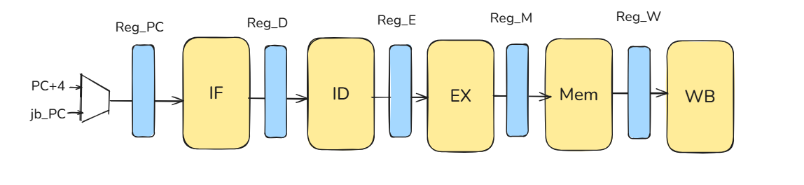
Pipeline registers are the boundaries that split a long combinational datapath into stages (IF/ID/EX/MEM/WB). Each register latches data and control between stages so multiple instructions can overlap in time while preserving correct program order.
What they carry
source operands (or store data), immediates, rd/rs1/rs2, PC/PC+4 (as needed), and all control bits required later. Carrying control forward lets a younger instruction act correctly several cycles after decode.
11.2 Performance Analysis: Benefit and Cost
11.2.1 Frequency Benefit vs. Register Overhead
When we pipeline a processor, we cut the combinational logic into smaller stages. Ideally, this allows for a massive increase in clock frequency. However, this benefit comes with a cost: Pipeline Register Overhead.
The clock period of a pipelined processor is determined by the slowest stage plus the overhead of the registers:
\[ T_{\mathrm{clk}} \approx \max_i (\text{Stage Delay}_i) \;+\; t_{\mathrm{overhead}} \]
Where does the overhead come from?
Because we insert pipeline registers (Flip-Flops) between stages to latch data, we incur specific timing costs:
- Propagation Delay (\(t_{pcq}\)): The time it takes for the Flip-Flop to output valid data after the clock edge triggers.
- Setup Time (\(t_{setup}\)): The time the input signal must be stable before the next clock edge arrives for the next Flip-Flop to capture it correctly.
Therefore, the total overhead added to every stage is:
\[ t_{\mathrm{overhead}} = t_{pcq} + t_{setup} \]
11.2.2 The Latency Paradox
A common misconception is that pipelining makes individual instructions faster. The opposite is true.
“Pipelining improves throughput, not each individual instruction.”
If we look at just one single instruction, pipelining actually makes it slower (\(L_{\mathrm{pipe}} > L_{\mathrm{single}}\)).
From IF to WB, the total time increases because the signal must now traverse \(N\) pipeline registers, accumulating the overhead (\(t_{pcq} + t_{setup}\)) at every stage boundary.
So why do we do it?
We don’t optimize for a single instruction; we optimize for the flow of millions of instructions. We must look at Frequency and Maximum IPC (Instructions Per Cycle) simultaneously:
\[ \text{Performance} = \text{Frequency} \times \text{IPC} \]
- Frequency (\(\uparrow\)): By shortening the critical path to just one stage depth, \(T_{\mathrm{clk}}\) drops significantly, allowing the clock to run much faster.
- Ideal IPC (\(\approx 1\)): In an ideal pipeline, we finish one instruction every cycle.
Even though each individual instruction takes slightly longer (latency \(\uparrow\)), the rate at which we complete them (throughput) skyrockets.
11.2.3 Quantitative Analysis: Iron Law of Performance
To prove mathematically that pipelining reduces execution time, we use the classic Iron Law of Performance:
\[ \text{CPU Time} = \text{Instruction Count} \times \text{CPI} \times \text{Cycle Time} \]
Let’s compare the time to execute a benchmark program with N instructions (\(IC = N\)) on a Single-Cycle machine versus a 5-Stage Pipeline.
Setup:
- Stage delays:
[10, 6, 6, 10, 3] ns - Register overhead (\(t_{\mathrm{reg}}\)):
1 ns
Case A: Single-Cycle Machine
In a single-cycle design, the clock period must be long enough for the signal to pass through all stages in one go.
- Cycle Time (\(T_{\mathrm{single}}\)): \(\sum D_i = 10+6+6+10+3 = \mathbf{35 \text{ ns}}\).
- CPI: 1 (by definition).
- Total CPU Time: \[ \text{Time}_{\text{single}} = N \times 1 \times 35 \text{ ns} = \mathbf{35N \text{ ns}} \]
Case B: 5-Stage Pipelined Machine
In a pipelined design, the clock period is limited by the slowest stage plus the register overhead.
- Cycle Time (\(T_{\mathrm{pipe}}\)): \(\max(D_i) + t_{\mathrm{reg}} = \max(10, 6, 6, 10, 3) + 1 = 10 + 1 = \mathbf{11 \text{ ns}}\).
- CPI: 1 (Ideal, assuming no stalls).
- Total CPU Time: \[ \text{Time}_{\text{pipe}} = N \times 1 \times 11 \text{ ns} = \mathbf{11N \text{ ns}} \]
Comparing the two designs:
- Latency per Instruction:
- Single: \(35\) ns
- Pipeline: \(5 \text{ stages} \times 11 \text{ ns} = 55\) ns (Slower!)
- Throughput / Total Execution Time:
- We calculate the Speedup by dividing the total execution times: \[ \text{Speedup} = \frac{\text{Time}_{\text{single}}}{\text{Time}_{\text{pipe}}} = \frac{35N}{11N} \approx \mathbf{3.18} \]
The Cycle Time reduction (35ns \(\to\) 11ns) drastically reduces the total CPU Time, outweighing the latency penalty.
While we gain massive throughput, pipelining is not free:
- Higher Latency per Instruction: An instruction takes longer from IF to WB due to accumulated register overhead (\(N \times t_{\mathrm{overhead}}\)).
- Hardware Cost: Extra area and power consumption for the pipeline registers.
- Complexity: We must design units to handle hazards (Stall/Flush/Forwarding) to maintain valid IPC.
- Misprediction Penalty: Deeper pipelines mean more wasted cycles (bubbles) when we guess a branch wrong.
11.2.4 Control point for correctness
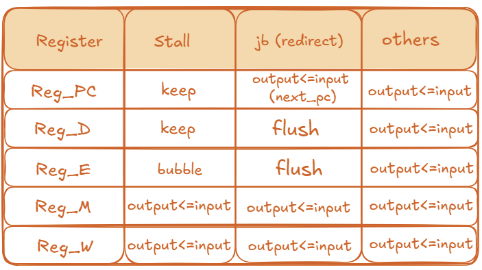
Pipeline registers are where we apply hazard control:
- stall: hold PC and IF/ID (keep =
output ≤ output) to wait for data; - bubble / flush: write a NOP into ID/EX (bubble) or into IF/ID and ID/EX (flush on redirect) so wrong-path or too-early work has no architectural effects.
Control policy
- stall: a one-cycle hold (typically the load–use RAW case). Pause the front end until data can be forwarded.
- jb (redirect): control-flow change (taken branch/jump or misprediction). Flush younger wrong-path ops.
- others: normal operation (no stall, no redirect).
- keep (
output ≤ output): hold the register value; do not advance this stage. - flush (
output ≤ nop): convert this stage to a NOP (no architectural effects). - bubble (
output ≤ nop): intentionally insert a NOP at this stage so older stages can drain.
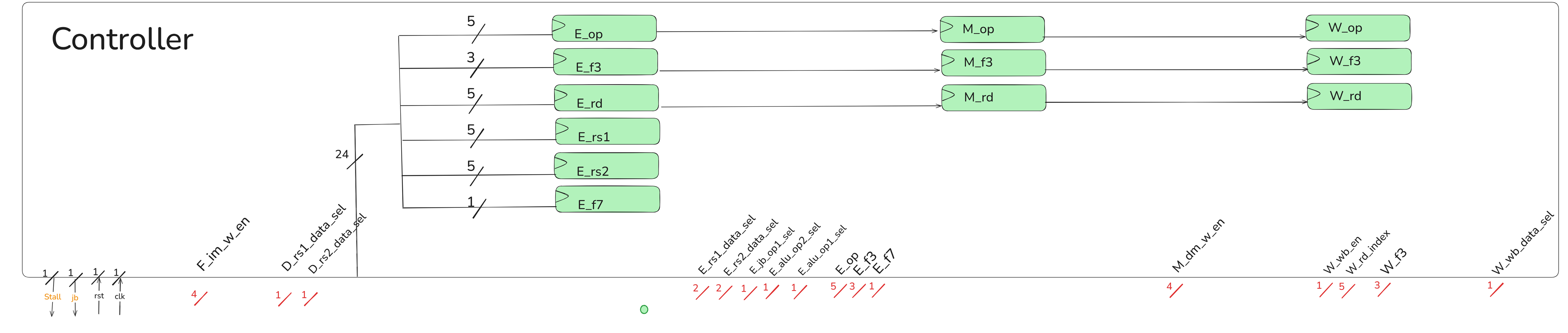
11.3 Controller
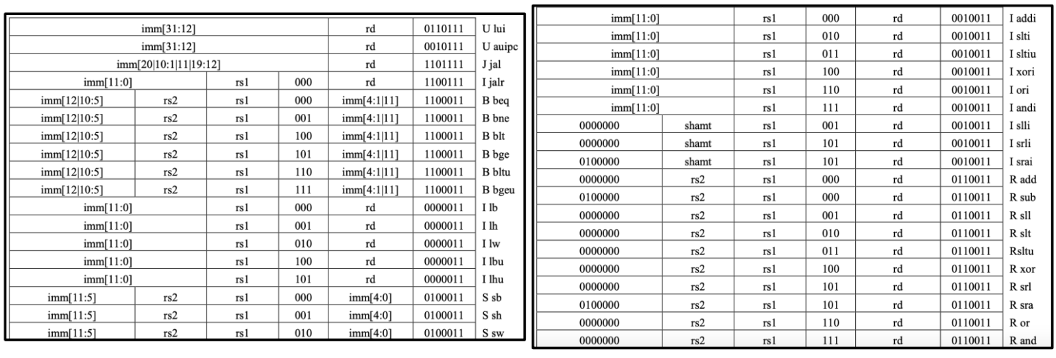
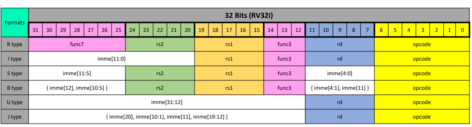
First, we will provide the RV32I instructions along with the corresponding type table for students to reference, followed by a presentation of the overall CPU block diagram. After that, we will introduce the purposes of the control signals.
11.3.1 RV32I Instructions
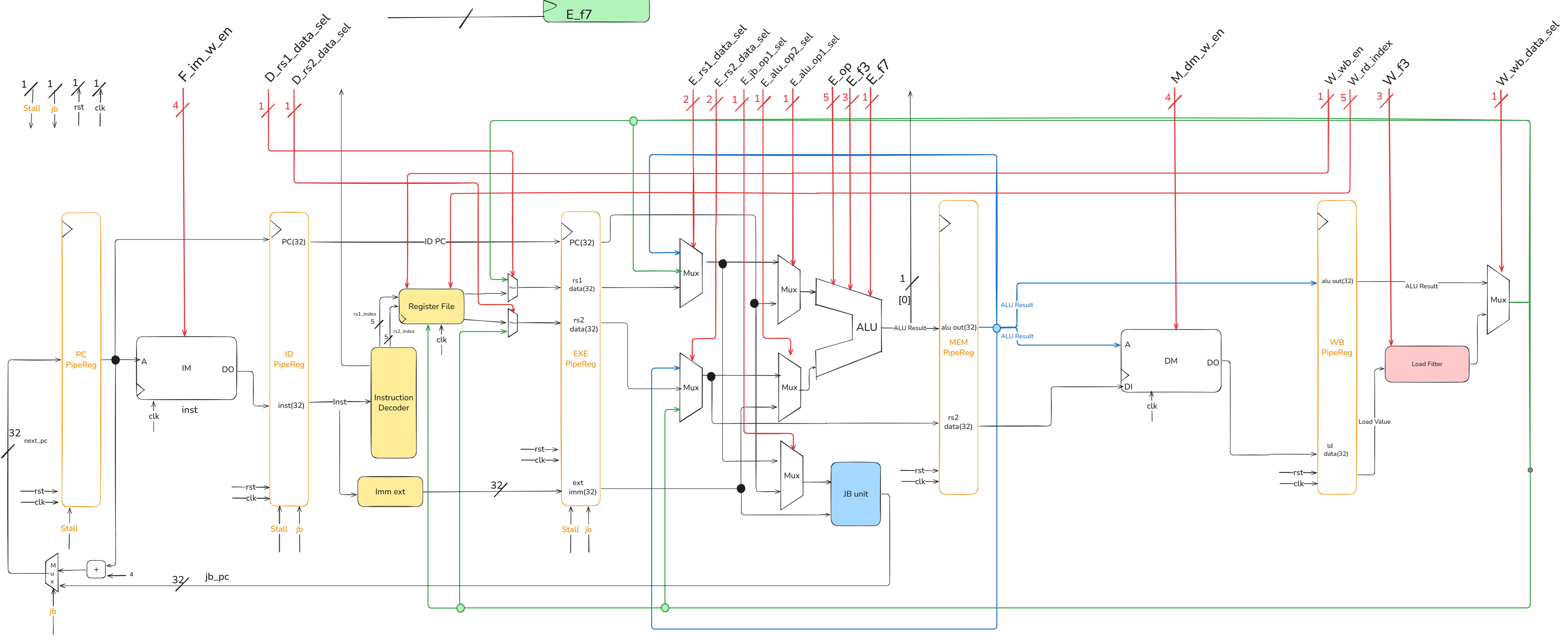
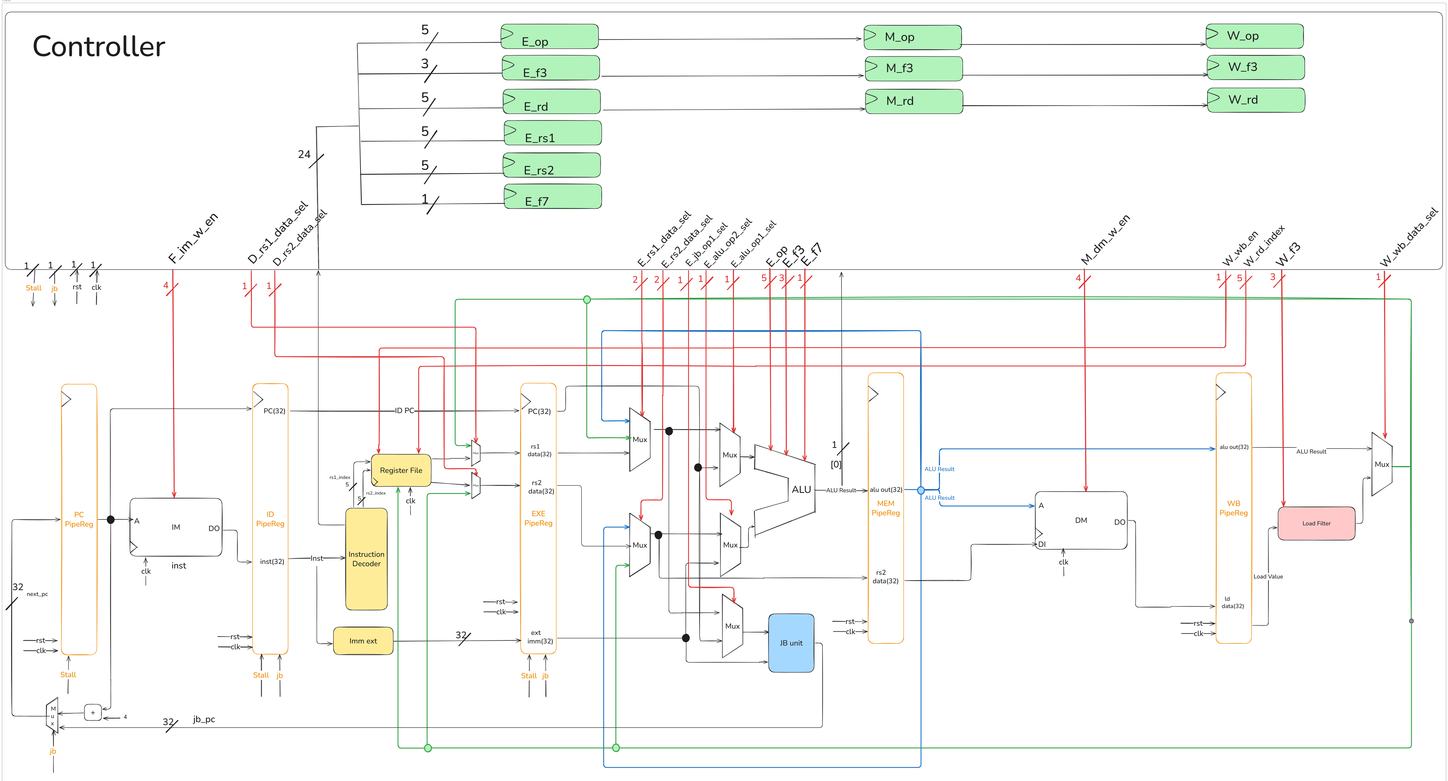
11.3.2 CPU Block Diagram
架構圖的memory要改成lab3的ROM,這裡由學長改動!!!!
特別檢查放大時,圖片畫質是否模糊,我是從畫布複製貼到小畫家再輸出成圖片檔,這樣放大也能清楚呈現圖片!!!!
The jb signal can also be viewed as next_PC_sel.
Since ALU_Result[0] is related to determining the jb signal, this signal needs to be brought out and provided to the controller.
If any part of the image is unclear, please zoom in as needed.
11.3.3 Control Signal
Need add some registers to keep instruction info in each stage and use the instruction info kept in each stages to get the control signals in each stages.
The number in parentheses represents the bit-width of the signal.
| Signal | Usage |
|---|---|
| F_im_w_en (4) | Prevent writing data into im |
| D_rs1_data_sel (1) | Immediately Read the Writeback rs1 data |
| D_rs2_data_sel (1) | Immediately Read the Writeback rs2 data |
| E_rs1_data_sel (2) | Get the newest rs1 data |
| E_rs2_data_sel (2) | Get the newest rs2 data |
| E_alu_op1_sel (1) | Select alu op1 (rs1 / pc) |
| E_alu_op2_sel (1) | Select alu op2 (rs2 / imm) |
| E_jb_op1_sel (1) | Select jb_unit op1 (rs1 / pc) |
| E_op_out (5) | Output the opcode in E stage to ALU |
| E_f3_out (3) | Output the func3 in E stage to ALU |
| E_f7_out (1) | Output the func7 in E stage to ALU |
| M_dm_w_en (4) | Store [ byte / halfword / word ] into dm |
| W_wb_en (1) | Whether write back data into RegFile |
| W_rd_index (5) | Write back register destination index |
| W_f3 (3) | Output the func3 in W stage to LD_Filter |
| W_wb_data_sel (1) | Select writeback data(ALU Result / Extended Load Data) |
| stall (1) | Set when there is a Load instruction in E stage and there is an instruction in D stage that uses the Load’s writeback data |
| next_pc_sel (1) | Set when a jump or branch is established in E stage |
The following code from Controller.v is provided to help explain the control signals.
D_rs1_data_sel & D_rs2_data_sel
Controller.v
E_rs1_data_sel & E_rs2_data_sel
Controller.v
Controller.v
stall
Controller.v
The is_E_use_rd flag can be optimized out due to redundant conditional checks.
11.4 The Essence of Predicting a Branch
In a pipelined processor, the Fetch stage must know the address of the next instruction to fetch in the very next cycle.
- For sequential instructions, this is simple:
Next PC = Current PC + Instruction Size. - For control-flow instructions (like branches), the next PC is not sequential. It could be the next sequential instruction (if Not-Taken) or a new Target PC (if Taken).
This is the Control Dependence problem. Waiting for the branch to execute (many cycles later) to know the correct address would cause the pipeline to stall, severely hurting performance.
A complete branch prediction mechanism must therefore guess two key things before the branch is even decoded:
- Branch Direction: Will the branch be Taken or Not-Taken?
- Branch Target PC: If it is Taken, what is the target address it will jump to?
Implicitly, it must also guess if the fetched instruction is a branch at all.
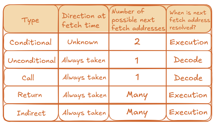
11.4.1 Types of Branches
Different branch types resolve their next fetch address at different times:
11.4.2 The Cost of a Misprediction
The penalty for a wrong guess is high. If a processor has N pipeline stages and can fetch W instructions per cycle (a “W-wide” superscalar processor), a single misprediction wastes \(N \times W\) instruction slots.
11.5 How to Predict Future Branches
We can broadly categorize prediction strategies into two types: Static and Dynamic.
11.5.1 Static Approach
Static prediction strategies are fixed, either hardwired into the processor or determined by the compiler. They do not adapt to the program’s runtime behavior.
- Always Predict Not-Taken:
- This is the simplest possible strategy. The hardware always assumes the branch will not be taken and continues fetching sequentially at
PC + Instruction Size. - Advantage: Extremely simple. No hardware is needed to store history.
- Disadvantage: Accuracy is very low (around 30-40% for typical programs).
- This is the simplest possible strategy. The hardware always assumes the branch will not be taken and continues fetching sequentially at
- Other Static Approaches:
- Always Predict Taken: This is slightly more accurate, as loop branches are very common and are “Taken” most of the time.
- BTFN (Backward Taken, Forward Not-Taken): A simple heuristic. Most backward-pointing branches are part of loops (so predict Taken). Most forward-pointing branches are for
if-then-elselogic (so predict Not-Taken). This is more accurate than the other simple static methods. - Profile-Based: The compiler runs the program once with a sample input to “profile” its behavior. It then adds a “hint” bit to the branch instruction in the final code to tell the hardware which direction is more likely.
The main weakness of all static approaches is their inability to adapt. If a branch’s behavior changes, the static prediction will be consistently wrong.
11.5.2 Dynamic Approach
Dynamic predictors use hardware to store the recent history of branches and adapt their predictions based on that history.
11.5.3 The Last-Time Predictor (1-bit Predictor)
The “Last-Time Predictor” is a simple dynamic predictor that uses a single bit for each branch. This bit is often stored in a structure called a Branch History Table (BHT) or as part of a Branch Target Buffer (BTB) entry.
- Mechanism: The single bit indicates which direction the branch went the last time it was executed.
- Prediction: The predictor guesses the branch will go in the same direction it went last time.
- Update: After the branch executes, the 1-bit entry is updated with the correct outcome.
The logic for a 1-bit predictor can be represented by a simple 2-state state machine.
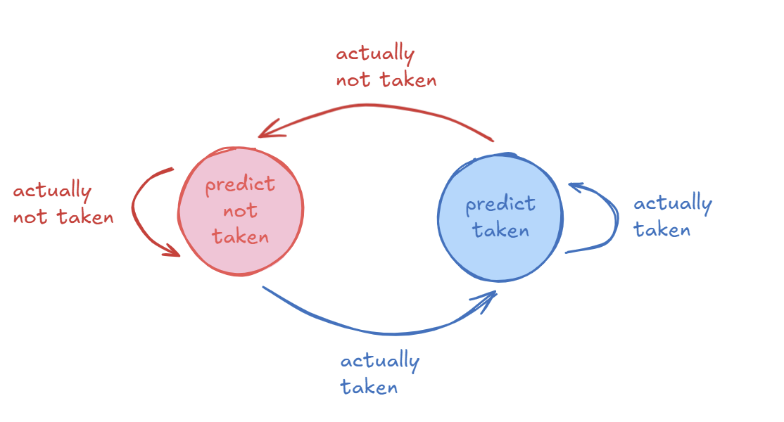
- Predict Not Taken State (0):
- If the branch is actually not taken, it stays in this state.
- If the branch is actually taken, it transitions to the “Predict Taken” state.
- Predict Taken State (1):
- If the branch is actually taken, it stays in this state.
- If the branch is actually not taken, it transitions to the “Predict Not Taken” state.
- Good Case: For a branch with a stable, repetitive pattern like
TTNNNNNNNNNN(Taken twice, then Not-Taken 10 times), this predictor is highly accurate (e.g., 90% in this case). - Bad Case (Loops): The predictor always mispredicts the first and last iteration of a loop. For a loop with N iterations, its accuracy is (N-2) / N.
- Worst Case: For an alternating pattern like
TNTNTNTNT..., the 1-bit predictor will achieve 0% accuracy because it is always predicting based on the previous outcome, which is always different.
The main issue with the Last-Time Predictor is that it changes its prediction too quickly. A single different outcome (like the last iteration of a loop) can flip the prediction, even if the branch is “mostly taken” or “mostly not-taken”.
11.5.4 Two-Bit Counter Based Prediction
To solve the problem of the 1-bit predictor changing too quickly, we can add hysteresis.
- Idea: Use two bits to track the history for a branch instead of just one. This allows the predictor to have “strong” and “weak” states.
- Mechanism: Each branch is associated with a two-bit counter. This counter uses saturating arithmetic, meaning it stops at maximum (11) and minimum (00) values.
- Hysteresis: The extra bit provides hysteresis. A “strong” prediction (like
11- Strongly Taken) will not be changed by a single different outcome. It requires two consecutive mistakes to flip the prediction from Taken to Not-Taken (or vice-versa).
This predictor uses a 4-state state machine. The prediction is based on the most significant bit.
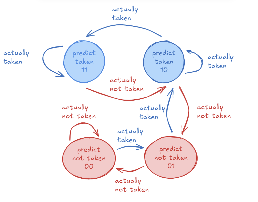
- States:
11: Strongly Taken (Predict Taken)10: Weakly Taken (Predict Taken)01: Weakly Not-Taken (Predict Not-Taken)~00: Strongly Not-Taken (Predict Not-Taken)
- Transitions (Example from
11):- If the branch is actually taken, the state remains
11(saturating). - If the branch is actually not taken, the state changes to
10(Weakly Taken). The prediction is still “Taken” but is now “Weak”. It takes another “Not-Taken” outcome to move to state01and change the prediction.
- If the branch is actually taken, the state remains
- Good Case (Loops): For a loop with N iterations, the accuracy improves to (N-1) / N. It only mispredicts the final exit.
- Bad Case: For the alternating
TNTNTNT...pattern, the accuracy is 50% (assuming it starts in a weak state). This is much better than 0%. - Overall: This predictor (also called a “bimodal predictor”) provides better accuracy than the 1-bit scheme.
- Advantage: Better prediction accuracy.
- Disadvantage: Higher hardware cost (e.g., more bits in the BTB entry).
11.6 The Architecture of a Complete Branch Predictor
A real predictor must solve all parts of the problem simultaneously. It does this with two main hardware structures.
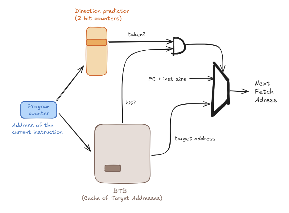
11.6.1 Branch Target Buffer (BTB)
- Purpose: To answer the questions: “Is this a branch?” and “If so, what is its target address?”
- How it works: The BTB is a small, fast cache.
- Indexing: It is indexed by the
PCof the instruction being fetched. - Entry: Each entry in the BTB stores:
- The
Target PC(the address to jump to). - The direction prediction bits (e.g., the 2-bit counter).
- The
- Indexing: It is indexed by the
- In Operation (at Fetch stage):
- The
Current PCis sent to the BTB. - If it’s a BTB Hit: The hardware predicts this is a branch. It reads the
Target PCand the 2-bit counter from the BTB entry. - If it’s a BTB Miss: The hardware predicts this is not a branch and sets the Next PC to
PC + Instruction Size.
- The
11.6.2 Branch Direction Predictor
- Purpose: To answer the question: “Taken or Not-Taken?”
- How it works: As described above, this is the set of 2-bit saturated counters. In a common design, these counters are stored inside the BTB. When the BTB hits, the 2-bit counter is provided along with the target address.
11.6.3 Putting It All Together: The Full Flow
- The
Current PCis sent to the BTB. - The BTB is checked for a matching entry (a “hit”).
- Case 1: BTB Miss
- Prediction: Not a branch.
- Next Fetch PC =
Current PC + Instruction Size.
- Case 2: BTB Hit
- Prediction: This is a branch.
- The
Target PCand the2-bit counterare read from the BTB entry. - The 2-bit counter’s state (e.g.,
11,10,01,00) determines the Direction Prediction (Taken or Not-Taken). - If (Predicted Taken): Next Fetch PC =
Target PC. - If (Predicted Not-Taken): Next Fetch PC =
Current PC + Instruction Size.
11.7 How to Handle Control Dependences?
Branch prediction is not the only solution. We have several strategies to handle branches:
- Stall: Pause the pipeline until the branch is resolved. (Very poor performance)
- Guess: This is Branch Prediction.
- Delayed Branching: The N instructions after a branch (in the “delay slot”) are always executed.
- Predicated Execution: Convert the control dependence into a data dependence.
- Multi-Path Execution: Fetch from both possible paths.
- Fine-Grained Multithreading: Switch to another thread.
11.8 Lab 4 Assignment
11.8.1 What You Must Do To Complete The Assignment?
There are two parts you must complete in the assignment:
- The program part — 80% of scores
- Assignment Report — 20% of scores
Program
Based on the Lab 3 single-cycle CPU, the following Verilog files are required to implement the Lab 4 pipelined CPU architecture:
- Top.v
- DEF.sv
- ALU.sv
- Decoder.sv
- Imme_Ext.sv
- JB_Unit.sv
- LD_Filter.sv
- RegFile.sv
- Adder.sv
- MUX2.sv
- MUX3.sv
- Controller.sv (you need to complete)
- Reg_PC.sv
- Reg_D.sv (you need to complete)
- Reg_E.sv (you need to complete)
- Reg_M.sv (you need to complete)
- Reg_W.sv (you need to complete)
- ROM.sv
- RAM.sv
- TextBuffer.sv
- Halt.sv
- CoreTop.sv
After completing the pipeline CPU, your RTL code needs to pass the ISS. At this point, compared to the single-cycle CPU, you will encounter the problem of pipeline bubbles:
The pipeline bubble will lead to the synchronization issue between ISS (which can be viewed as a single-cycle CPU) and pipeline CPU.
We might have to extend previous reference-model-based verification framework to adapt to pipeline CPU and add some check flags to notify the verification framework to stop ISS and wait for the completion of Pipeline CPU.
For example, you can add a bubble signal from the WB stage. When the WB stage executes a NOP instruction generated due to a stall or a jump/branch, this bubble signal is asserted to stop the ISS and wait for the pipeline CPU to catch up.
Report
Your report should demonstrate your understanding of pipeline hazards and your specific implementation strategy. Please answer the following questions:
For each hazard (Forwarding case, Load-Use Stall, and Control Flush), describe:
- Trigger Condition: Under what specific circumstances does this hazard occur? (e.g., Which specific instruction sequence? Which register indices are compared?)
- Resolution Strategy: How does your hardware resolve this hazard? (e.g., Forwarding data, inserting a bubble, or flushing the pipeline?)
- Implementation Logic: How did you implement this in
Controller.v?- For Forwarding: How do you decide priority if multiple stages have the data?
- For Stalls: Which pipeline registers are held (frozen) and which are flushed?
- For Branches: How do you clear the wrong-path instructions?
- Branch Prediction
- Please carefully study the branch predictor section of the handout. If it were up to you, which branch predictor design would you choose (Static vs. Dynamic, 1-bit vs. 2-bit)? Why?
- Describe how you would design the control signals to resolve the control hazard caused by mispredictions (e.g., logic to flush instructions in IF and ID stages). (Note: Implementation is bonus, but the conceptual description is required).
Bonus ( + 20 points)
In your pipeline CPU RTL code, you must implement the branch predictor and show in the report that the total clock cycles decrease. You also need to submit an additional version of your pipeline CPU RTL code that includes the branch predictor.
11.8.2 Steps To Prepare for Doing Lab 4
Compile